

KeyStrategy
has a 7 year history. It has emerged as a need for a group of traders for internal use, whose functions have gradually evolved according to the current need. Now, the program is accessible to you so far in the beta release for control and interface, which has been redesigned for simple and logical control of the public version so it is user-friendly. The KeyStrategy is still ready to develop and we welcome all constructive reminders. You can write to our support.
Software and hardware requirements:
Software: Windows 10, 64 bit version.
Minimal hardware requirements: 2 GByte RAM, 2 cores Intel i5
recommended hardware requirements: 8-32GByte RAM, 4 cores and more Intel i7 or Xeon 6 cores and more
Data Source:
The data market resource natively uses a high-quality SierraChart database that favors high-quality data at an affordable price. You can also use exported data (.txt format) from Tradestation and NinjaTraders, which also features high-quality data with a long history. If you work with stocks long-term strategies and you would like to have daily bars, you can use Quandl data with a long history free of charge. For the public version, we plan to add support for additional data sources, but we recommend the sierrachart data for the best performance.
Now let’s start:
Here are some quick instructions: how to Install
In the example of creating a simple strategy, we show the program’s control and the appropriate workflow. Run KeyStartegy. If you do not see the blue KeyStrategy log window go to the “Charts / Open Workbook“. Enter the name of the new strategy in the New WorkBook field. Press Create. A chart window is created. The Workbook can contain more Charts (“Charts / New Chart“). You can also create any number of Workbooks, but you can only have one open. If you want to open a new Workbook, the current one is automatically closed.
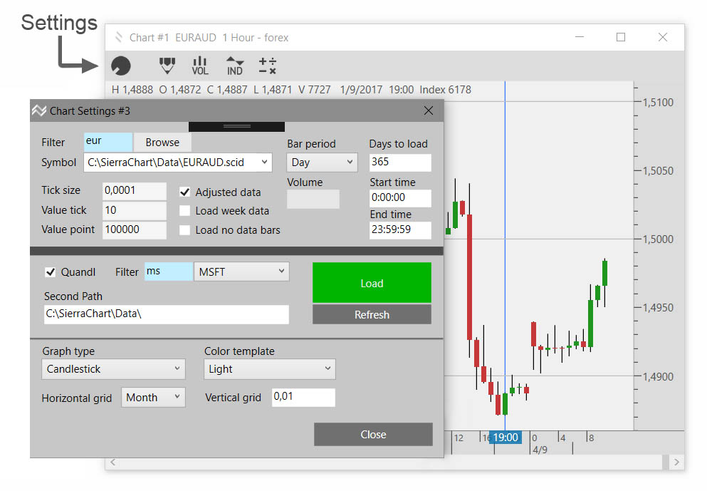
In the Chart window, go to “Settings” and set:
- The market symbol on which you want to test the strategy. Use “Filter” for a large number of items, or just type the symbol without a path in the “Symbol” box or press “Browse” to select the market directly on the disk (You can change the market at any time)
- Number of days, for example 365 if you want to test for a 2 year sample of data.
- Timeframe, such as 1hour.
- Display style, such as Candelstick.
Press “Load”, it should load and plot the price chart. In order to retrieve the data, it must be stored either in the installation folder “.\ Data \” or in the “Second Path” folder which you can set in the Second path field. For example, if you use SierreChart as the data source, type “C: \ SierraChart \ Data \” directly into Second Path field. -more-
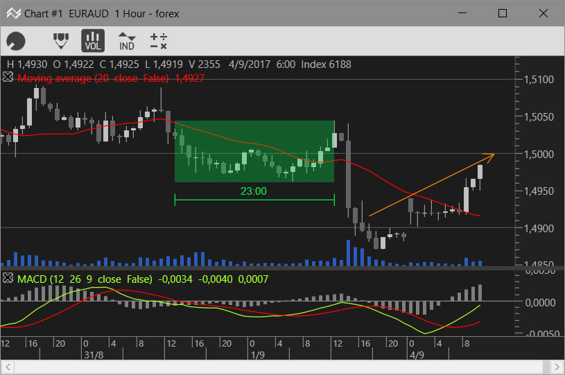
In the Chart window, we can control the graph view:
- Right mouse button can move the chart in all directions.
- Right mouse button in the vertical ruler area by moving up and down to change the zoom.
- Double-click in the vertical ruler area to set the fit to vertical zoom and move the graph to the last bar.
- Use the left and right buttons to move the chart. Up, down the horizontal zoom.
At the top there is an icon bar:
- Sketch: you can write and draw notes on the chart. -more-
- Volume: Turn on a simple volume graph directly in the pricing chart without using the indicator. To open the volume chart with a ruler, open it as an indicator.
- Indicators: Add the indicator to the chart. -more-
- Strategy: Choose the strategy you previously created and want to test. If you do not have your strategy yet, you can first select one of the demo strategies, and press OK. (In the main “Tools / Strategy” menu, open a window where you can create and edit strategies.) -more-
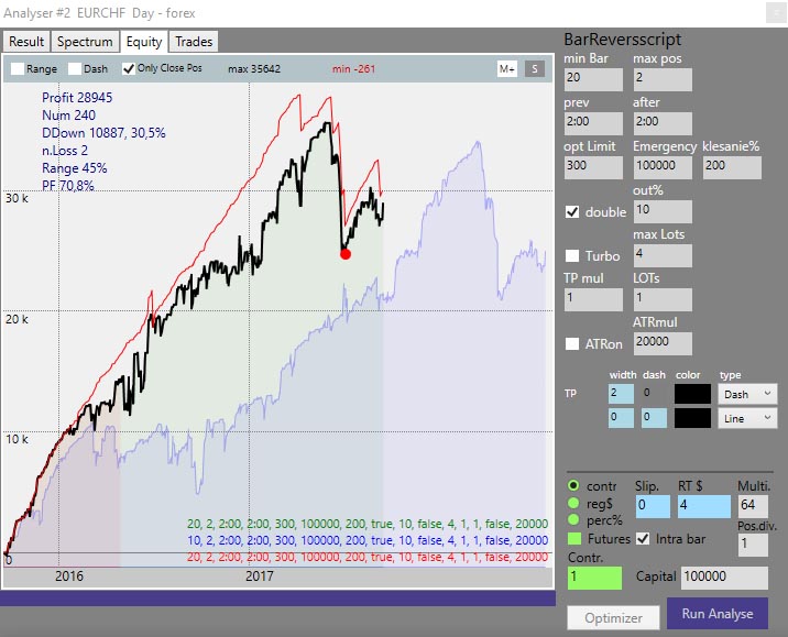
Analyzer: If you choose a strategy, the Analyzer window opens. On the top of the page are the tabs that show each result of the backtest: Result, Spectrum, Equity, Trades. On the right, there is a strategy parameters column that you can change. Press Run Analyze to run Backtest.
In tabs you can see the results:
- Result: Shows profits, losses … individually for Long positions, Short positions and all together. Very important are the %Drawdown and ProfitFactor parameters.
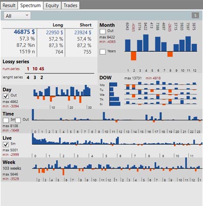
- Spectrum: Here are the statistical graphs such as time success in the month or year, the success of each day of the week, the lifetime of the trades over time, You may look at the total statistics or statistics for each year. From the monthly chart we can see seasonal dependence if we have a sufficient sample of data. -more-
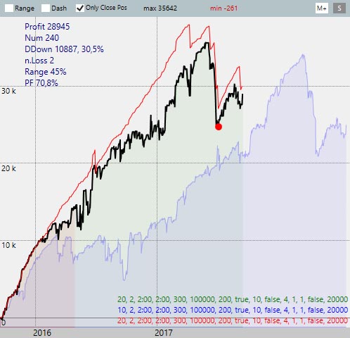
- Equity: One of the most important chart. From the course of equity, you can see the character of your strategy in more than it seems at first glance. Equity can be stored as “Ghost” and after changing parameters or adjusting the logic to see how the curve has changed. These “Ghosts” can have more in the graph, it is a very powerful tool in creating and fine-tuning your trades idea. -more-
- Trades: Listing of individual trades. By double-clicking on a particular trade, you can go to the trade location on the chart.
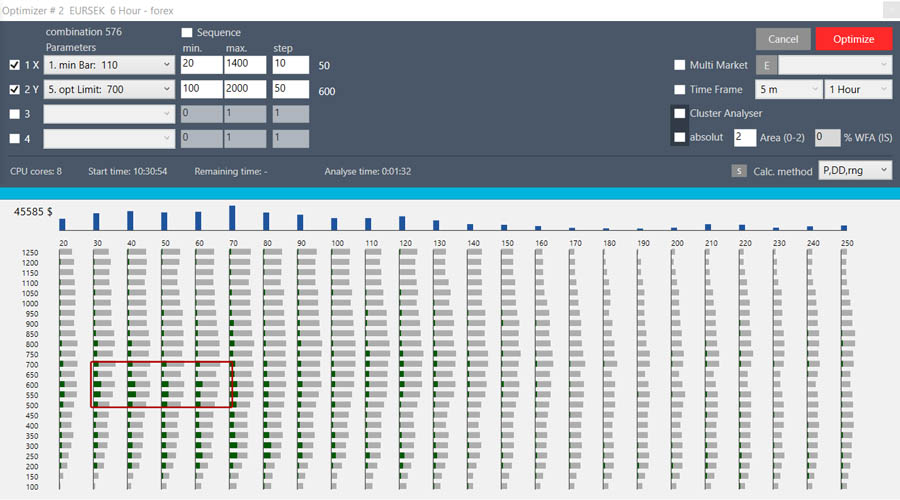
Optimizer: If we complete our strategy and the code is final, we can fine tune the individual strategy parameters to the best possible result, according to the different evaluation schemes. The number of optimized parameters at once should be as small as possible, ideally from 1 to 3. The program deliberately limits this number to a maximum of 4. The parameters we optimize together should be logically related. Common optimization of a large number of unrelated parameters leads to pre-optimization! (values of parameters that produce good results by accident, but are in fact not tradable, such a system will not work in the real world and may cause losses on the account). KeyStrategy has effective means of detecting such situations. -more-
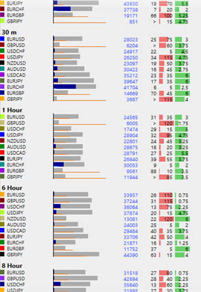
Multi Market Optimization (MMO): You can optimize your new strategy on groups of multiple markets. You can create these groups yourself. For example, the technology sector in stocks, Commodity Grains, or Forex Major Pairs. If our strategy is robust enough, it should have similar results across all markets in that group. If many markets in the group do not work or go into a loss, it means that our strategy is not robust enough.
The illustration is an example of a strategy that did not stand within a given group of markets. Too many markets have failed.
Multiple markets optimization can automatically test not only the entire market group but also each market for a specified range of TimeFrame. Using MMO, you test not only the robustness of the strategy, but you also find new markets that might be suitable for your strategy. By trading multiple markets on one strategy, you can diversify the risks within one strategy. Using MMO in multiple markets and timeframes will save you tremendous amount of time to develop and test your strategy.
Walk Forward Analysis (WFA): It is a very powerful tool for testing robustness and detecting the risk of pre-optimization. Parameter optimization takes place only on part of the data sample (InSample “IS”) and the rest is backtesting from the calculated parameters (so-called Outsample “OS”). The Equity Chart will show us a blue area that represents the future. If the course of equity in this area breaks down or deteriorates significantly, it means that the strategy is inappropriate. WFA works with the MMO module and can test the whole set of data at once. On the external equity chart, I’ll show all the charts together. If the curves on the wfa break evenly into the vegas, (some continue the trend of others going to lose) it means that the strategy probably has no edge. (see Fig.) -more-

WFA Cluster Analysis: No test is perfect, the future can not be predicted, our best chance to succeed in the markets lies in maximizing testing and verifying the functionality of our system in the most comprehensive backtest with a long history. Have you gotten through the optimization of the most suitable parameters, followed by MMO and WFA testing here and you are satisfied with your result? WFA Cluster Analysis is still ahead. It analyzes the whole map of wfa analyzes with different IS-OS ratios and different depth histories in the relative and absolute raster. All tests are automatically evaluated and result in a Heat Map.
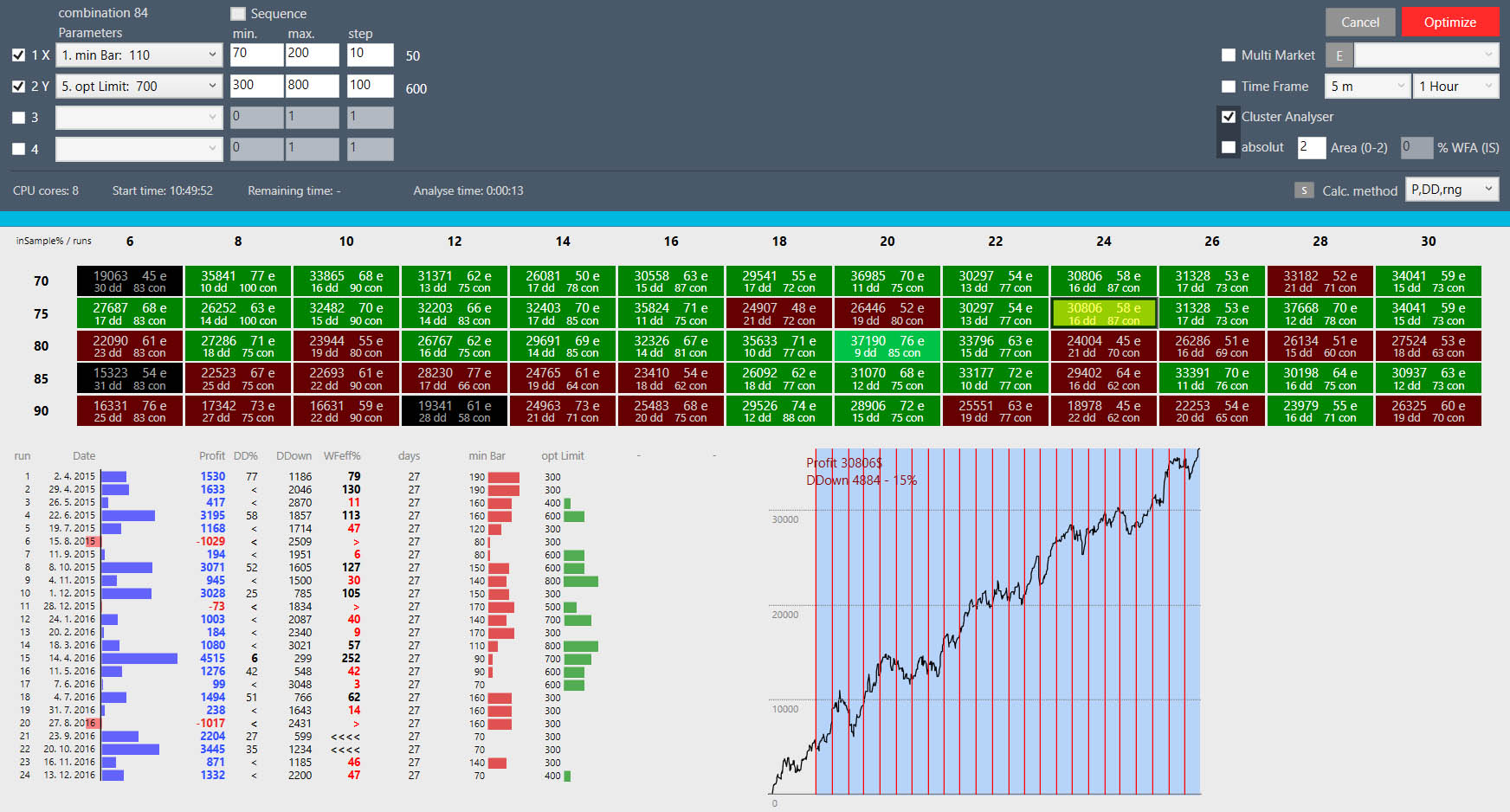
The whole process is very demanding, thanks to the unique KeyStrategy algorithm and full multi processors support, it takes a tenth of time compared to the classical process. The heat map must have a large enough green field. Black and red boxes are unsuitable, the best are pale green. If the Heat map is about 1/3 of the red or black or green field is not quite complete (the checkerboard turns green fields with red or black) it is a sign that your system is not robust enough. You can click on each Heat Map box and show us the entire test series of the cluster. Individual optimization periods, calculated parameters and final WFA graph. It is up to you to dive into the study of results such as the development of the values of a certain parameter over time, or rely on the color of the Heat Map. For example, you can use the average value of a parameter over a certain period. Achieving the ideal result on the WFA Cluster analysis is not at all easy. But when we get a good result, we can say that in the field of testing, we have made our system the most. -more-
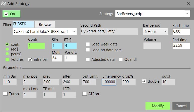
Portfolio manager: Diversify your risks. The more strategies you trade in multiple markets, the better your diversification. You have much more time to respond if one of your strategies stops working without fatal consequences on your equity. In portfolio managers, you can arbitrarily combine your strategies, markets, timeframes, position sizes, and parameters. It is good to combine different types of strategies to reduce our Total Equity Drawdown. Add New Portfolio: create a new portfolio, enter a name and description. Duplicate, Delete: Duplicate or delete selected portfolios. Create Equity: Start the calculation of the entire portfolio. In a separate window, you will see Equity of the entire portfolio plus equity of individual strategies. At the top of the rows are the results of individual strategies (profit, drawdown etc …). We also have Ghost memory, Snip, Range capabilities same as in the Equity window analyzer. Days to load: the length of history. Copy, Paste: You can copy items between individual portfolios. Add New Startegy: adds a new strategy to the portfolio (opens new “Add Strategy” window) Delete, Edit: Erase or modify the selected strategy in the portfolio. At the bottom of the window is a listing of individual strategies with a given name, timeframe, and parameters. Rows that are grayed off, they can be edited but not taken into the calculation. This way, we can easily test the appropriate combinations.
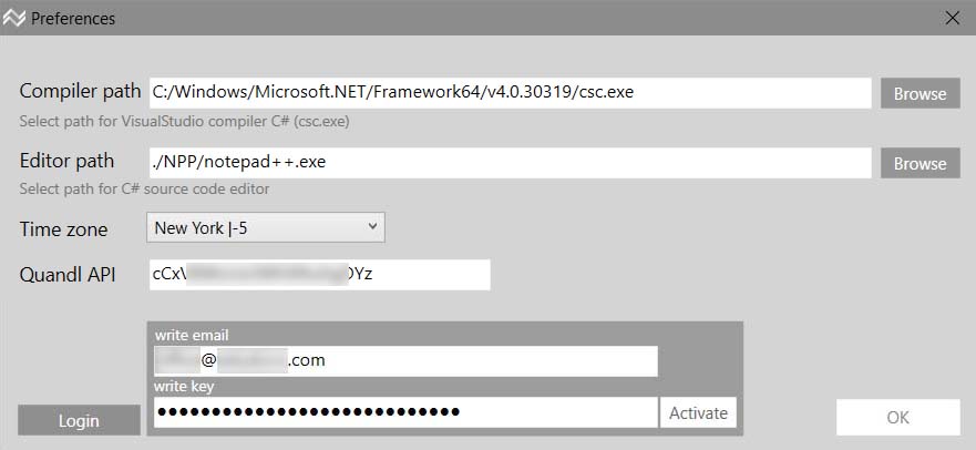
How to install: After the order (for free) you will receive a mail with the order information and a download link. You can also find this link on the Account / orders section of the website. After downloading and installing the program go to “Tools / Preferences”
- Press the Login button and enter the email and activation code you find in the order email. Press Activate.
- After the successful activation, the Login Successfull message appears in the pop-up window and the Activate button will be green. If the red activation button is not running (you are not connected to the internet, you entered a bad email or the code or program expired)
- In the Compiler path field, you have to set the path for C# compiler. -more-
- In the Editor path, you can change the path to the strategy code editor. We recommend using the supplied editor.
- Time zone: Set the time zone for your region.
- Quandl API: Register for free at www.quandl.com and get the API code you will be writing here. You can then use Stock Daily data for free.
Example data setting in Sierrachart:
- Download and install the program. https://www.sierrachart.com/index.php?page=doc/SoftwareDownload.php
- In the “Help / Acount Control Panel“, set up and purchase Service Pack 3.
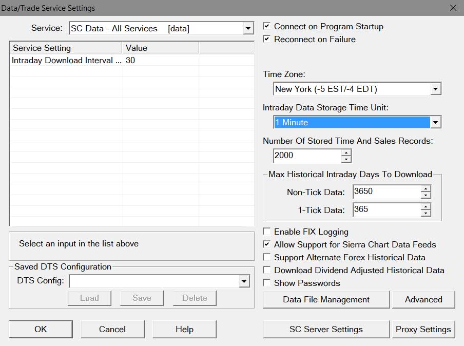
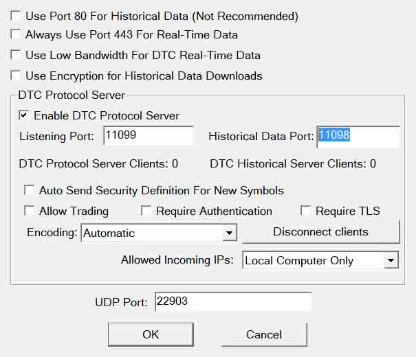
- In the “File / Data-Trade Service Settings“, set the data according to the pictures.
You can set “Service” on your Broker (for example, Interactive Brokers). You can then trade – place a orders directly from the graph. “Max Historical Intraday Days To Download” determines the maximum depth of history to upload. Alternatively, you can enter other values. Depending on the provider, what a deep history is available for that market.
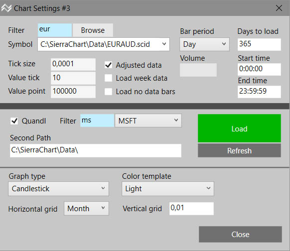
We set market, format, and display style in chart settings. Filter: write the starting letters 1 and more than the filter for faster search. Symbol: In the scrolling list, we can select a given market. (markets are searched for “./Data/” and SecondPath) If we know the exact symbol we can write it straight (without suffix). In this case, the search directory for the “./Data/“, then Second Path folder is searched, and finally, trying to retrieve from an external source (for example, SierraChart or Quandl if the checkbox Quandl is enabled). If the disk data with a shorter history how is required then the program tries to retrieve data from an external source. Using Browse, you can choose any data file from the disk. Tick size, Value tick, Value point data are automatically set according to the selected market. If you used the non-standard symbol name, these values will need to be filled by yourself. The manually edited fields will be blue. Bar Period: Time Frame from 1 second to 1 month. Timeframe under 1 minute is only possible if we have tick data. Time Frame Volume and Range are exotic formats that we recommend using only exceptionally if it has some logical sense for that strategy. If we select Volume or Range TF, we still have to fill under the “Bar period”. “Volume”: Number of trades per bar, “Range”: Maximum bar height (price range). These formats also require tick data, we also seeing with a minute data, but then we only have to measure only with the information value of such charts. Days to load: the number of days that will appear in the chart. Load week data: if uncheck does not load weekend data (Saturday, Sunday, midnight to midnight). Beware of data that will be omitted depends on the selected time zone! Load no data bars: create those bars where there was no trade. Start time, End time: You can only load a certain part of the day. This feature is only suitable for intraday transactions. Beware of changing the value of the indicators! Default is set all day. Load: load the set symbol. Refresh: When connected to an external data source, it uploads new data. Market saved on disk will be updated. (applicable to SierraChart and Quandl) Quandl will prefer data from the Quandl source. The filter accelerated our search from the list of markets provided by Quandl. If a market is selected we will automatically copy it to “Symbol”. At the end of the table there are options for styling the chart.
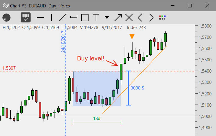
Activate drawing by pressing the pen in the top bar or by pressing the D key. Select tool: Press and hold the left mouse button and drag the selected tool. H – Horizontal (price) line. V – Vertical (data) line. L – Trend line. P – Ruler. Depending on the direction of drag, it measures the price or time. R – Area. Mark the area. T – Text. We can write notes in the chart. M – Marker. By dragging, we can change the marker type. A – Arrow.
Click on tool, we can select the tool. The checkpoints appear. You can move points using the mouse or arrow keys. We will delete the tool with Del (Del) or X icon. You can change the selection using the arrows in the toolbar. If you hold the Control key using the Up, Down, Left, Right keys, we can change the color, thickness, frame (Area), and size (Text). Cancel the drawing by pressing the pen or Escape key.
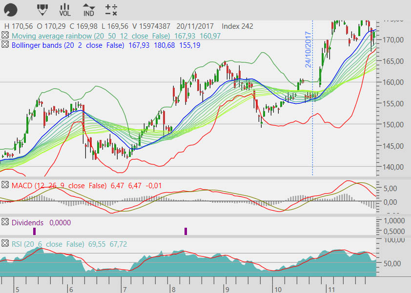
On the top bar of the chart, press the IND icon. A window opens with a selection of available indicators.
KeyStrategy provides the basic types with which you are rich. Indicators exist countless, but their principles are mostly the same and do not bring any added value. By endlessly scanning the lots of indicators, we will not get anything, but you will lose a lot of time. It is important to remember that each indicator is only a mathematical derivative of the price we see on the graph. This implies that it is difficult to find a significant edge in a strategy built on one simple indicator. Of course this does not mean that the indicators are unnecessary. Indicators have their irreplaceable place in trading, but many beginner traders put them in too much importance as they really do. Indicators have significant additional help and orientation guidance in the price chart. Your strategy can use values from indicators. In strategy, however, you can also create custom indicators that are logically related to your strategy, using internal results, and appearing in the chart as a normal indicator (in this case the “A” icon). If required, it is possible to add additional versions in the next releases. In the Indicators window, double-click the indicator. On the right, you can set parameters and styles of views. Below the list, you can set the row position (1 = price chart). Press OK. The indicator in the graph has an “X” icon on the top left. Left mouse click to close the indicator. The right mouse click opens a small window where you can change parameters and style. Confirm change with the Enter key. Scale, fit, and scrolling work just like the price chart. There may be more indicators in one row. It is not advisable to combine the indicators in one window with too different values because the vertical scale is of course common to all of them at once.
Analyzer: In the Chart window at the top bar, touch the strategy (+: – x) icon. Select a double-click strategy. If you have not yet, you can still use demo strategies already in the program. WARNING! Demo strategies are here for learning purposes only and they are not complex strategies ready for trading. Demo strategy, of course you can start editing by yourself. Press OK. The Analyzer window opens. On the top are tabs “Result, Spectrum, Equity, Trades”: Result: shows the results of the analysis.
Spectrum: The Spectrum module can reveal the time dependence of the success of our strategy within different time periods. The accuracy of these statistics greatly depends on the length of history we are testing
- Year: Select the year or all of the strategy. You can compare the success of each year.
- Month: Monthly results. The seasonal dependency of the strategy may be demonstrated (if we test for a sufficiently long history). Check “Out” trades will rank in stats by closing date, otherwise open. “Years” will show the results in the month and for each year separately. The results over the years should not jump too much. Lossy series: list of series in a row.
- Day: results within the month.
- DOW: results within a week and in a table even during the year. The beginning of the week may be weaker, and so on.
- Time: the success of the day’s stores.
- Live: Duration according to the duration of the trade.
- Week: Weekly results. Each chart has its maximums (min, max) in order to have an idea of what drawdown we can expect in the month, weekend … Using the Sprectrum module, we get a valuable idea of what results and “surprises” we can expect from your Strategy.
Equity: Equity is one of the most important graphs that we are about to build. He’s seeing a lot about the nature of our Strategy.
- Range: Shows the range of volatility, which is an important indicator used for example when optimizing.
- Dash: Display style.
- Only Close Position: The red equity curve shows only closed trades. Black shows real equity (we can have many open positions that are currently in a loss or profit).
- M +: We can memorize the progress of equity and, after changing the parameters or the code, we can compare what changes have caused. Equities will appear in the graph as “Ghost” and the parameters that were used. Click on the line of parameters at the bottom of the chart to delete the corresponding “Ghost”.
- S: We can also take all the equity into any number of separate windows. These are also copied to the clipboard and you can put them in your notes in Excel.
- In the top left graph, baseline data is displayed from the “Result” table.
Trades: Chronological listing of all trades. Double-click on the relevant trade to move to a place in the price chart where the trade started. It will be marked with a red arrow. The Index column is the price bar number. For example, we can use this index as a breakpoint in the code when fine-tuning the strategy. On the right, you will see the strategy parameters, the graphical settings of each field, and a standard setting that you need to check and set up for each strategy separately: Position size: (green area)
- Contract: Set absolute value (1 means one Futures Contract, 100 Shares for Shares, 1 Lot (100,000) for Forex)
- Reg $: The position size will be automatically set so that the stoploss has a specified value (200 means 200 $ stoploss)
- Perc%: The position size will be automatically set so that stoploss has been given percentages of the capital.
- Futures: will set positions only for whole numbers (futures contracts), for stocks and forex leave unchecked.
- Capital: the amount of capital. (using Perc% and Cluster Analysis).
Slippage: (blue area) predicted sliding. Standard 1. Too volatile markets, markets with small volumes, high spreads may also have a much larger slip. It is important to enter a real average slip of the market, preferring more than less. Markets with large slippage can make a loss-making strategy with a functional strategy. RT $: Commission size for the entire trade, ie purchase plus sales. Commission can also significantly influence the efficiency of the strategy. (save Ghost from Equity, change the value of the commission to zero, press “Run Analyze” and make sure how many the commission will affect your earnings). Multitrade: You can trade multiple positions together in a single strategy. (max. 64) These positions can be overlap. For example, we have 3 long positions after 2 contracts and 2 short after 3 contracts. The resulting market position is currently zero, but Stoploss and Takeprofit are still in the market, and we are back in the market after we complete them. Multitrade can limit the number of joint trades. Standard is 1. Position divide: We can still divide each position into multiple parts. Thus, in strategy we can have several Takeprofit. For example, we close the first third on the TP 50 tick, the second on the TP 100 tick, and the third on the TP 200 tick while moving SL to the BE. Standard is 1. Intra Bar: The strategy also takes into consideration the movement inside the bar. For example, even if we use Day TF, the Analyzer loads the lowest TF available (ideal tick, standard 1 minute which is 99% sufficient). In this way, the bar strategy can enter or exit the position several times in bar. The analysis is more accurate, considers for example the gaps between ticks that are otherwise covered in the bar. Of course, it is slower and more memory-intensive. It is not always necessary to use this feature. For example, if our TP and SL are bigger than the average height of the bar or only enter the marketBuy command at the beginning of the bar, then uncheck Intra Bar, your work will accelerate significantly. Run Analyse: starts the analysis Optimizer: open the optimizer window
Optimizer: Combination: the number of analyzes to be counted. 1X, 2Y, 3, 4: Turn on optimization slot, select parameter, set limits (min. Max.) and step. The maximum number of steps is limited to 24. It is unnecessary to optimize one parameter per 100-1000 increments, we just only increase the calculation time. Press “Optimize“, after the step column you will see the resulting parameter, below is the result table for each step (only for slot 1X and 2Y). The first row shows the average of the second parameter (for the whole column) for each step of the first parameter. The bars in the main table have two values, the gray is Profit and the color is the height of the evaluation parameter. The equity curve is displayed in a separate window. Sequence: optimization runs through slots. Not all combinations are passed, the first parameter is first optimized and the result is already used to optimize the next one. This method is suitable for parameters that are logically unrelated. Area: if you enter a value of 1 or 2, the optimizer will not look for the best single result but the area of the best results. It is good if similar results are found around the ideal value without major fluctuations. It’s also a form of protection against pre-optimization. Calc. Method: select the type of evaluation parameter.
- P, DD, rng: standard. When evaluating Profit, Drawdown, Range. The range parameter ensures that the strategy does not go too long on the side.
- Profit, DD: evaluating Profit and Drawdown.
- DDown%: only Drawdown is considered in the evaluation.
- P-DD: simple calculation of Profit – Drawdown.
- PLfactor: only Profit/Loss Factor is considered in the evaluation. Strategies with a small PL factor have poor robustness and high sensitivity to Slippage and commissions.
Multi Market: Optimization runs on a group of markets that you choose from the worksheet to the right. If you press “E” (next to the worksheet), the Market Groups window opens. Here you can create or edit your own groups of markets. If you press Control key the “New Group” button change to “Duplicate”, you can duplicate and then edit a new group.
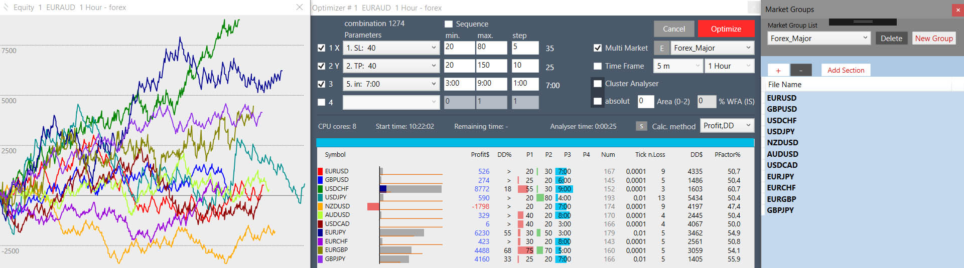
After optimization, a list of all results markets and a new window of Equities for each market together (color-coded) will be listed in the main window. Timeframe: If we mark TF, we can set the range of TF that each market should test. We can test multiple TFs on one market only and disable the “Multi market”. WFA (IS): To use Walk Forward Analysis, enter a percentage for the InSample (typically 50-80%). Standard is 0 – off Wfa. In an open equity chart, OutSample will be marked with a blue area. When using Wfa in Multi Market, the beginnings of equity graphs go forward to align the IS-OS edge, and clearly outweigh the impact of this break on each equity. Cluster Analyzer: Optimizer runs in Cluster Wfa mode. Heat map is colored by rating: the best is pale green, green, red, black. Each field contains: Profit (all OutSample zones), Wfeff% (Wfa efficiency, recovery rate ratio in IS and OS), Drawdown (should not be greater than 20%), the ratio between loss and profit time sector. If you click on the cluster box, you will see a list of the individual time slots with the resulting parameters and the equity curve with the marked area of the OS (blue area) and the time slots separated by the red line. Absolute: IS slots will have a precise time division by months.
Create Strategy:
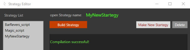
In the main “Tools / Strategy” menu, open a window “Strategy Editor” where you can create and edit strategies.
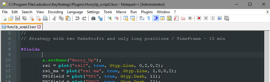
In the left column, double-click the strategy from the list. The strategy opens in a text editor that is selected in preferences. You can use any text editor.
Normally we recommend using the excellent text editor Notepad ++. Notepad ++ is free software and is pre-installed in KeyStrategy. For a newer version, you can download and reinstall it yourself from the https://notepad-plus-plus.org/download page.
When first launched Notepad ++ must be set in the menu “Settings / Style Configurator / Select theme: Obsidian” and in the menu “Language: KeyStrategy”.
The currently selected strategy is listed in “open Strategy name:”. If we have the code done or we have opened a demo strategy, we can compile it. Press the “Biuld Strategy” button. “Command Prompt” opens with the compiler message (csc.exe) whose path is set in preferences. Press the Enter key twice, the compiler window closes, and the “Compilation successful” message appears in Strategy Editor. In the event of an error, these are listed with the appropriate line number. If we remove the error, we’ll run the compilation again.
After successful compilation, the strategy appears in the “Chart / Strategy” menu. We can change the strategy code even while it’s in use! For example, save equity (Ghost), we make a change in the code, compile it, run “Run Analyze” again, and we can now compare the resulting change.
We are creating a new strategy:
Press the “Make New Strategy” button, type the name of the new strategy, press “OK”. The text editor opens a new strategy code with a pre-structured code and a simple example of a strategy that you can delete or edit as you like.
We write the first strategy code: Run the application. You have a description in the menu “Help / KeyCode”.